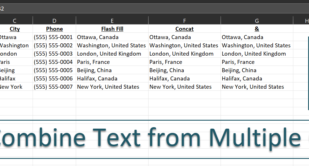
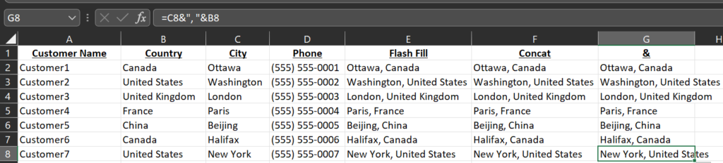
Today we will explore 3 ways of quickly combine text from multiple columns in Excel. In this example, we will combine the name of the City and the Country, while adding a comma in between. For example Ottawa, Canada.
Combine Text from Multiple Columns using Flash Fill
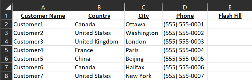
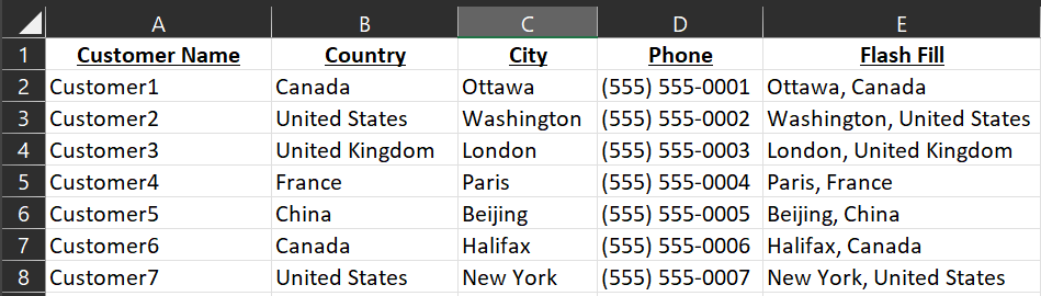
Excel 2013 introduced a new feature called flash fill, which seems to be getting better with every new release. Using the Customers – Exercise Book tab, we will be filling in column E, titled Flash Fill.
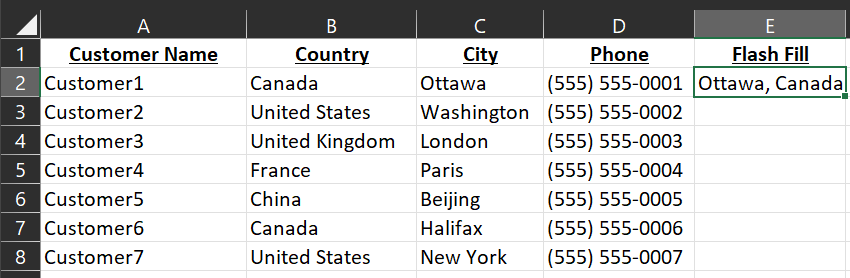
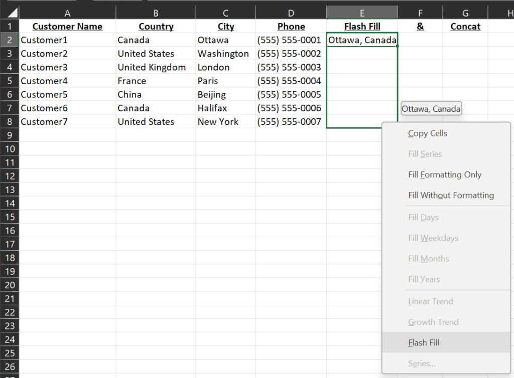
In cell E2, we will write the results how we would like to see them, in this case we will write Ottawa, Canada.
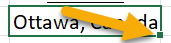
Next, we will select cell E2, and you can either press Control+E to fill in the rest of the column automatically, or you can right-click and hold the square in the bottom-right, and drag your mouse to the bottom of the table, as we can see here:
Select Flash Fill in the drop-down that appears. Excel’s AI will automatically fill in the rest.
Combine Text from Multiple Columns Using the Concat() function
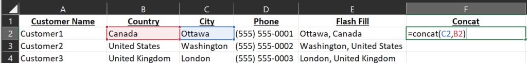
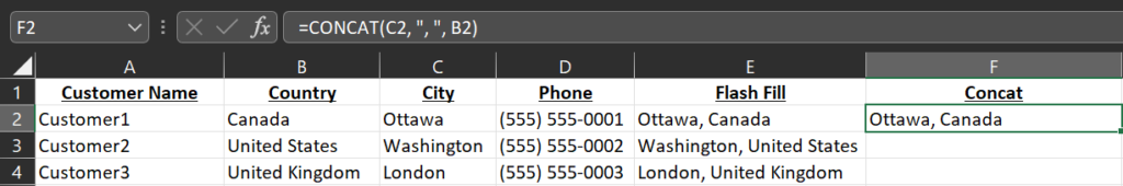
The Concat function can be used to combine data from multiple columns. In column F, we will do a quick formula to show how it works. We will start with concat(C2, B2), which will combine cells C2 and B2 together.
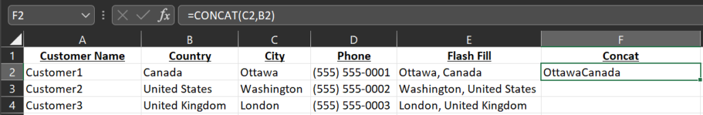
The end result is not quite what we want. As you can see, it squished both cells together, which we will fix next.
We will fix this by adding the text we want as a separator by using “, ” as follows: concat(C2, “, “, B2). As you can see, this formats the text as we expect it: Ottawa, Canada.
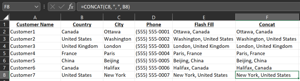
As always, you can drag the formula down by left-clicking the square in the bottom-right of cell F2 and dragging it to the bottom of the table to fill in the other cells automatically.
Combine Text from Multiple Columns Using &
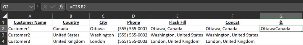
The last method we will see today is the one I actually use the most, which uses the & instead of the concat() function. To begin, in G2, we will write =C2&B2. Again you will notice that we get OttawaCanada all bunched up together. We will fix this in the next step.
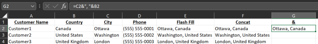
As we did with the concat() function, we will use “, ” to add a comma and a space between the City and Country, giving us the following formula: =C2&”, “&B2.
As always, you can left-click the square in the bottom right of the cell to drag down the formula to fill in the City, Country for the rest of the table.
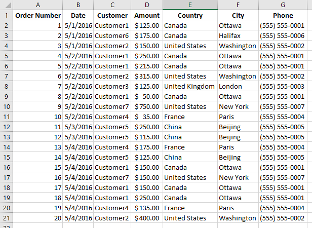
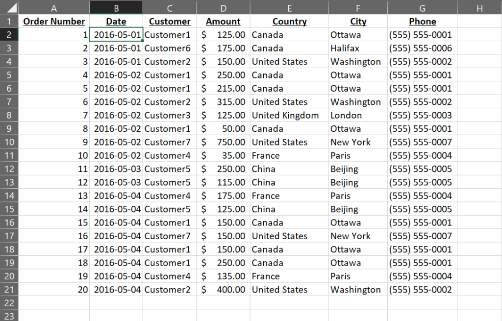
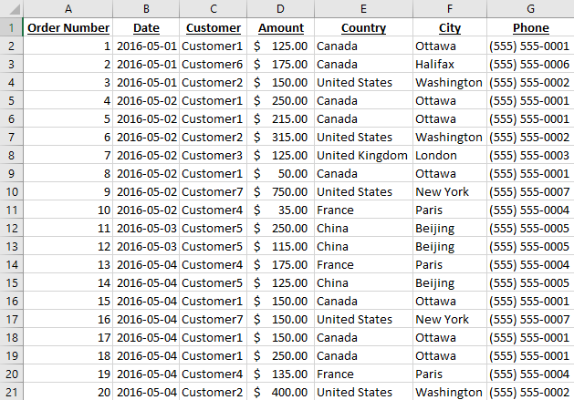
As an example of how the Excel Pivot Table feature works, let’s take a simple excel workbook with the following two tabs: Orders and Customers.
The Orders tab contains an order number, date, customer name, and amount. For the purposes of this exercise, we won’t be using the Customers tab.
To begin, select the entire table, from cell A1 through to cell G21, or click on any cell within that range.
Or
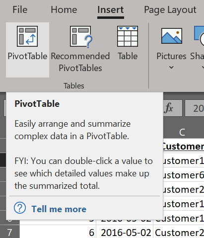
In the Insert ribbon, click the Pivot Table button.
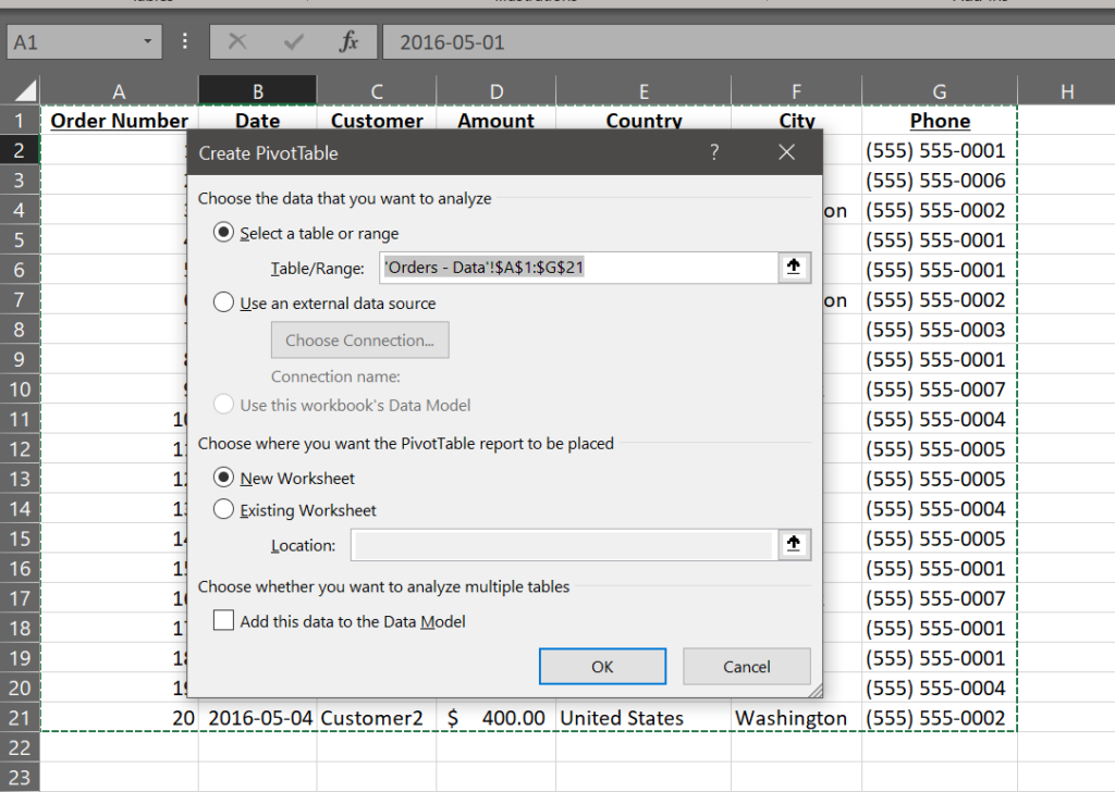
The Create PivotTable window will appear which shows the table/range that will be used as the input for the Pivot Table, and where you want the pivot table to be added.
In this case, we will keep the default, and use New Worksheet. Press OK to continue.
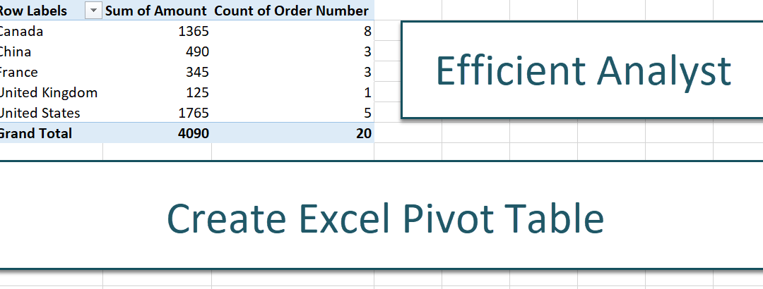
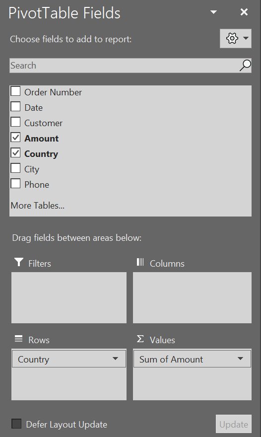
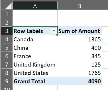
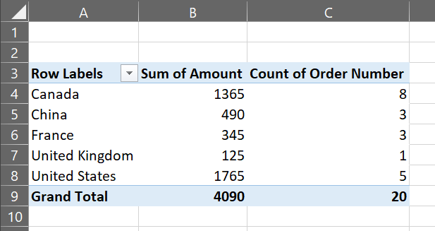
In the PivotTable Fields area, click and drag the Country field to the Rows section, and the Amount to the Values section. You will notice that Excel automatically notices the Amounts column contains numbers, so it will give you the sum.
Notice the results are now displayed on the left.
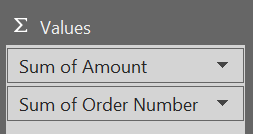
To add the count of orders, we will drag the Order Number field to the Values section also. Notice how Excel also detects the Order Number as a number, so chooses to aggregate with a sum. We will fix that shortly.
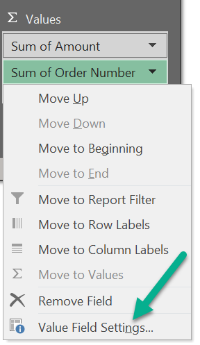
Click the triangle next to the Sum of Order Number, and select the Value Field Settings… menu option.
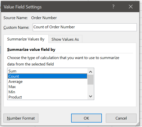
In the Value Field Settings window, select Count. This will rename the Custom Name as Count of Order Number.
Click OK to apply the changes, and see the final results.
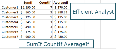
Using Sum(), Count() and Average() formulas in Excel might be enough for many situations, but sometimes you might have a more complex question you’re trying to answer. For example, if you had the following data, and you wanted to know how much each customer bought, how many times they bought, and what was their average purchase, you will need a new set of formulas. Don’t worry, though, you’ll see they are just as easy to use. The Excel SumIf(), CountIf() and AverageIf() formulas will give you the sum, count, and average of a value where a certain condition is matched.
To follow along, go to the following link to download the Efficient Analyst SumIf CountIf AverageIf Exercise Workbook:
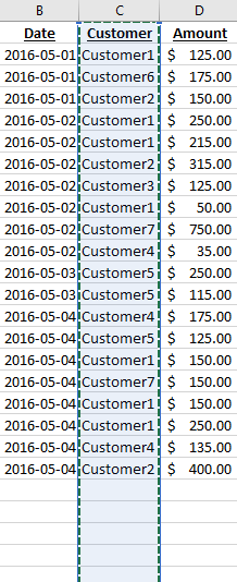
First, lets look at our sales data. You might recognize this from a previous exercise.
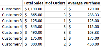
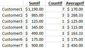
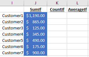
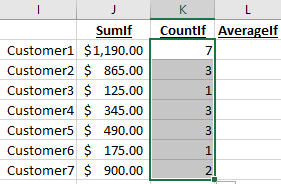
What you are looking for is a simple table as follows, so you can start learning more who your best customers are, and some of their buying habits.
Let’s see which functions will give us the right information for each column:
Using the Excel SumIf Formula
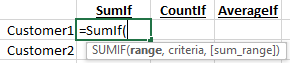
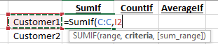
If you start writing =SumIf( in Excel, a tooltip will appear which gives you a reminder of how to use this formula.
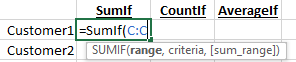
The first part you will need to fill out is the range. In this case, the range will can be thought of as “Where do you want to look for this customer name?”, the answer being column C, which in Excel you can either click the column C header to select it, or write C:C. Let’s click the column header to select it:
Also notice how the formula updated.
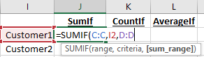
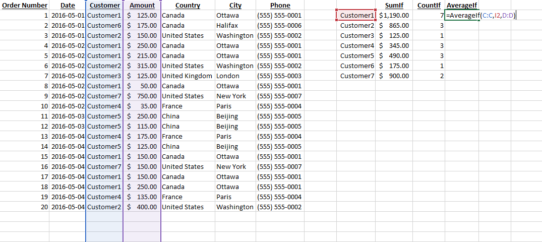
The second section we have to fill is the criteria. The criteria is what you are trying to match, which in this case is Customer 1, which is found in cell I2, so we will select I2.
Last but not least, we need to tell Excel what we need to sum, the sum range, which in this case would be the amounts found in column D.
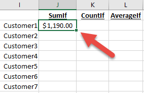
Congratulations, you know know how to use SumIf!. If you close the parenthesis ) of the formula and press enter, you will see how much Customer1 has purchased:
Dragging Down a Formula to Copy it Over a Range
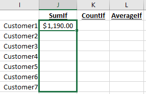
One of my favourite features of Excel is the ability to drag a formula down to copy it quickly over a range. Select the cell containing your SumIf formula, and then click and hold your left mouse button on the the little dot in the bottom right of that cell.
While keeping your left mouse button pressed down, move your mouse cursor down over the area you would like to copy this formula to.
Release the left mouse button, and you will see the formula copied itself over making adjustments as needed so the formula in cell J3 is matching the content in cell I3, etc.
Using the Excel CountIf Formula
To find out how many times each customer placed an order, we will use the CountIf formula, which counts how many times some text appears in your selection. This formula is a little simpler than the other two, having only two sections: a range, and a criteria.
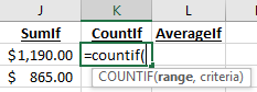
The first step consists in writing =countif( to see the Excel tooltip.
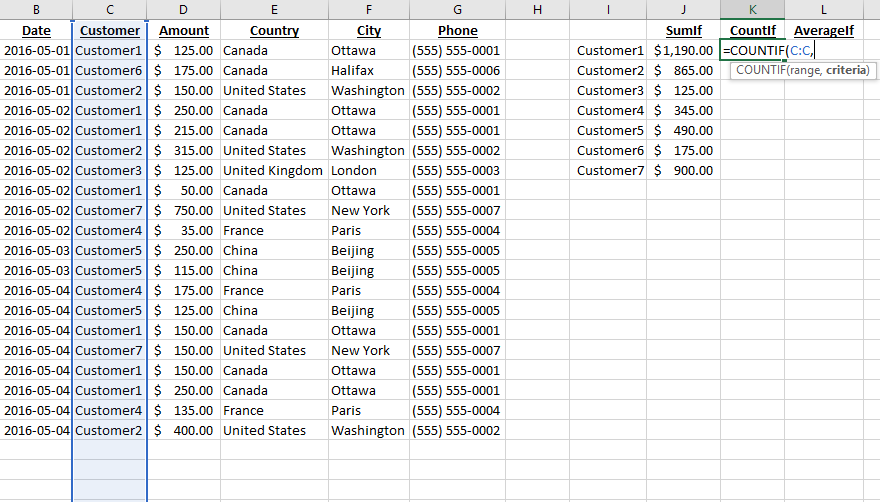
The range comes first, which is where you want to look for a match, which in this case would be column C. You can either select column C, or write C:C in the formula bar.
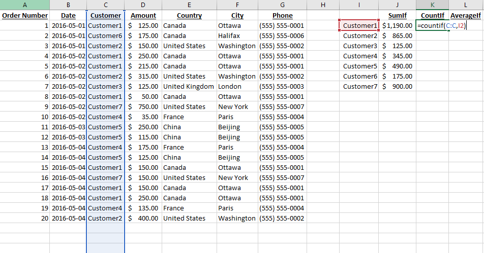
Next up is the criteria which is what we are trying to match, which in this case would be the content of cell I2.
Closing the parenthesis ), pressing enter, and then using the dragging technique from before, we get the number of purchases per customer.
Using the AverageIf Excel Formula
To obtain the average sales amount per order, we have two options. Since we already calculated the sum of the amounts and the count of orders, we could simply go in cell L2 and type =J2/K2. But since this is a tutorial, let’s use this exercise as an excuse to learn AverageIf, that way you don’t have to use SumIf and CountIf if all you’re looking for is the average.
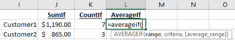
As usual, type =averageif( in a cell will give you the tooltip on how to use this tool. If you look at the 3 arguments of this formula: range, criteria, and average range, you’ll notice this follows the same structure as the SumIf() formula we have just seen.
Using a range of column C, a criteria of cell I2, and an average range of column D, we get the following formula:
Using the same drag-down technique as before, we get the average sales per customer.
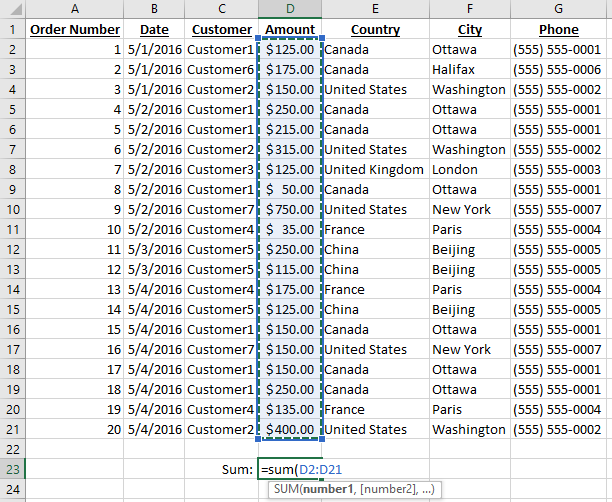
The Sum formula is a great one to start with. Excel formulas all start with an = sign, followed by the function name and a section in parentheses to provide ranges or arguments. Start out by typing =sum(
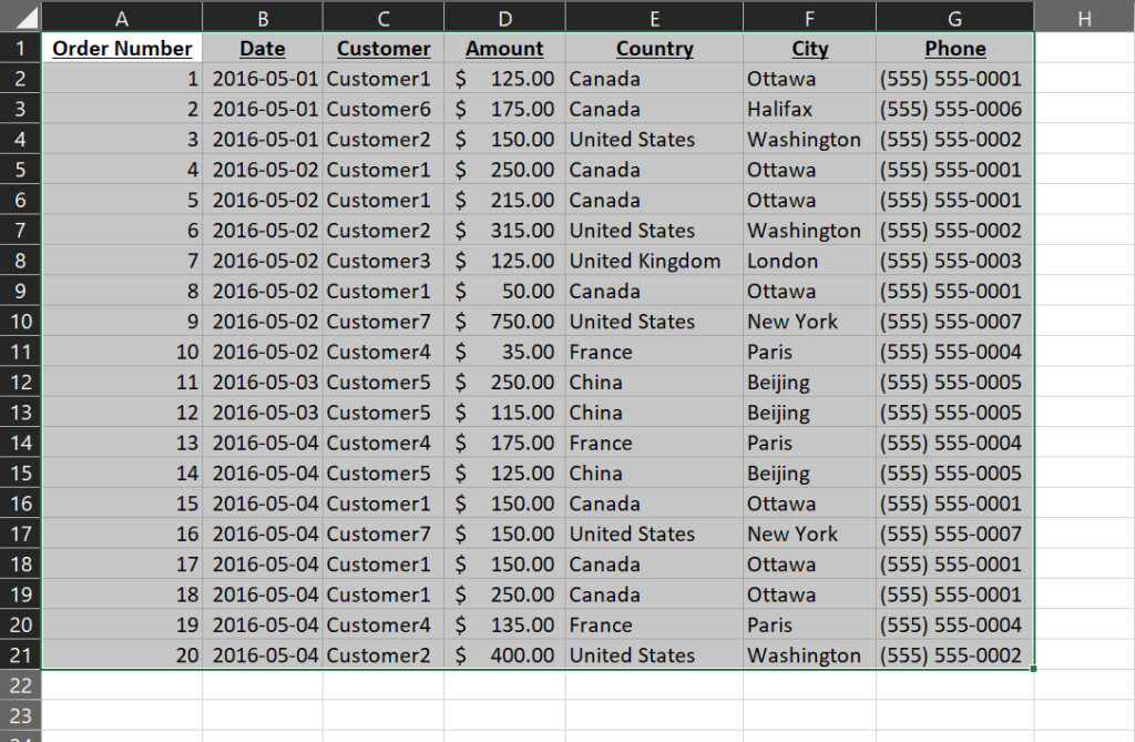
Sum requires a range of cells you want to add together. You can type your range in, or you can select it using your mouse or input device. In this case, we will select D2:D21.
Next up you can close the parenthesis, although newer versions of Excel will auto close it for you.
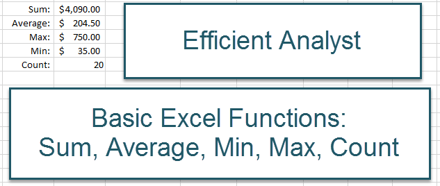
Excel Basic Formulas: Sum, Average, Min, Max, and Count
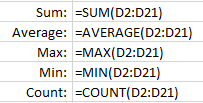
Using the same method, you can calculate the average, minimum value, maximum value, and count:
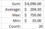
Which if you were using the downloadable exercise workbook, will give you the following results:
Here are some basic formulas, and what they do.
Sum
Adds all the cells together and gives you the total sum.
Average
Gives you the average of the selection you provide.
Min
Returns the smallest value from the selection you provide.
Max
Returns the largest value from the selection you provide.
Count
Counts how many cells have values in them.
Additional Tips
In the bottom right of the screen, newer versions of Excel provide you with a Sum, Average, and Count by default, and can be configured by right-clicking on it to provide minimum, maximum, and numerical count.
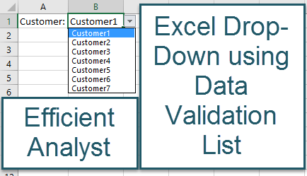
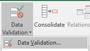
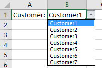
Adding an Excel Drop-down list is a great way to make data entry faster, more efficient, and also more accurate. There are a few ways they can be done, and in this article we show how to do them using the Data Validation lists.
As an example of how the Excel Vlookup function works, let’s take a simple excel workbook with the following two tabs: Orders and Customers.
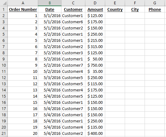
The Orders tab contains an order number, date, customer name, and amount.
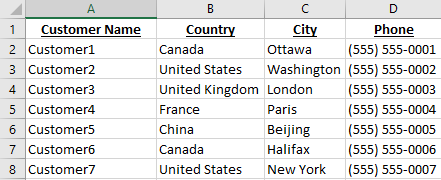
We want to add the Country, City, and Phone number of each customer, which thankfully we have in the Customers tab.
By using the Excel VLOOKUP function, we can quickly and efficiently fill in the Country, City, and Phone in the Orders tab.
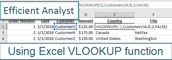
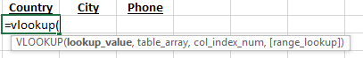
Let’s go back to the Orders tab, and start typing the =vlookup( formula to see the tooltip provided by Microsoft:
If you’ve never used the Excel vlookup function before, this provides absolutely no help. But lets break it down in an easier way:
Argument
Description
Example
Example Code
lookup_value
The value which is in common between both tables
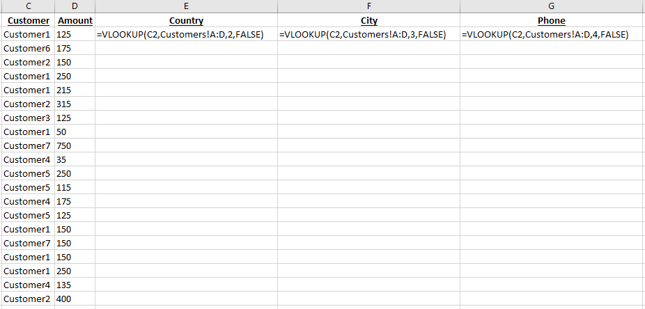
In this case, Customer Name, more specifically, if we are trying to find the Country for the customer on line two (i.e. we are trying to fill cell E2), we would select cell C2 as the customer name.
C2
tabble_array
Where the information you are looking for is located. The first column should contain the common element, and the range should be large enough to include
In this case, it would be the Customers tab, columns A through D.
Customers!A:D
col_index_num
Based on the range you put in table_array, the col_index_num is the number of the column which contains the result you are looking for. For example, if you selected A:D as your range, and the common element is in column A, and the result is in column B, you would put 2 as your column number. Putting 3 would give you the result from column C, and putting 4 would give you the result from column D. However, if you select L:P as your range, then column 1 is L, column M is 2, column N is 3, etc.
Because the country code is located in column B of the Customers tab, we will select 2
2
[range_lookup]
Last and definitely not least, the range_lookup gives you a true or false option. False will only return an exact match, while True will try to look for a result which looks similar to what you are looking for. 99%+ of the time I find False to be the best option to use. For example, if you had an order for Customer8, because there is no Customer8 in the customers tab, using false would return #N/A meaning Excel could not find a match. This would let you know that you have to add Customer8 to the Customers tab. If you select true, that same Customer8 would return United States, because Customer8 looks similar to Customer7, which is in the US.
false
We end up with the following formula: =VLOOKUP(C2,Customers!A:D,2,FALSE), where C2 is the Customer we are trying to match up, Customers!A:D contains the customer information we want to look into, 2 is the 2nd column from that range, and False because we only want exact matches.
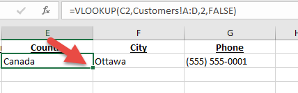
Using the same method, we can create the formulas for F2 and G2 by changing the 2 to a 3 or a 4. (I changed my view settings in Excel to show the formulas instead of the values, so you should see Canada, Ottawa, and (555) 555-0001 instead of the formulas)
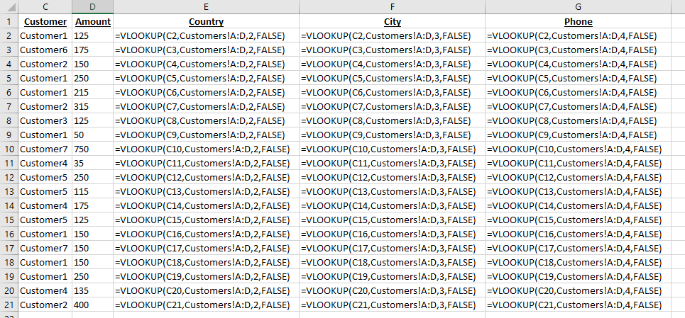
You can then select a formula and drag the little dot in the corner to fill in the other formulas very quickly:
Which would give us the following formulas (again in formula view):
Here is what you should see on your screen at the end. By using the formula dragging feature, you can very quickly perform vlookups for thousands of records!
Additional Tips
Using full columns as your range, for example A:D instead of A2:D7, makes it easier to add/remove items from your table without having to change the 2 and 7 all the time.
If you do use a range such as A2:D7, remember that if you drag your formula down, you will get A3:D8, A4:D9, etc, and if you drag your formula right, you will get B2:E7, C2:F7, etc. The easiest way to prevent this is to use $ signs to make sure the range doesn’t change, such as $A$2:$D$7.
We use cookies to ensure that we give you the best experience on our website. If you continue to use this site we will assume that you are happy with it.


Recent Comments