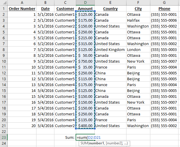
The Sum formula is a great one to start with. Excel formulas all start with an = sign, followed by the function name and a section in parentheses to provide ranges or arguments. Start out by typing =sum(
Sum requires a range of cells you want to add together. You can type your range in, or you can select it using your mouse or input device. In this case, we will select D2:D21.
Next up you can close the parenthesis, although newer versions of Excel will auto close it for you.
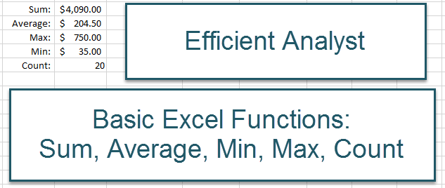
Excel Basic Formulas: Sum, Average, Min, Max, and Count
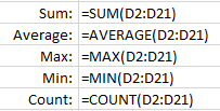
Using the same method, you can calculate the average, minimum value, maximum value, and count:
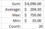
Which if you were using the downloadable exercise workbook, will give you the following results:
Here are some basic formulas, and what they do.
Sum
Adds all the cells together and gives you the total sum.
Average
Gives you the average of the selection you provide.
Min
Returns the smallest value from the selection you provide.
Max
Returns the largest value from the selection you provide.
Count
Counts how many cells have values in them.
Additional Tips
In the bottom right of the screen, newer versions of Excel provide you with a Sum, Average, and Count by default, and can be configured by right-clicking on it to provide minimum, maximum, and numerical count.
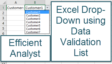
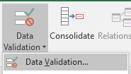
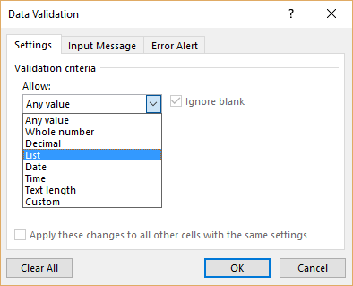
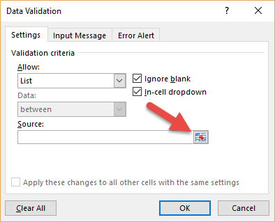
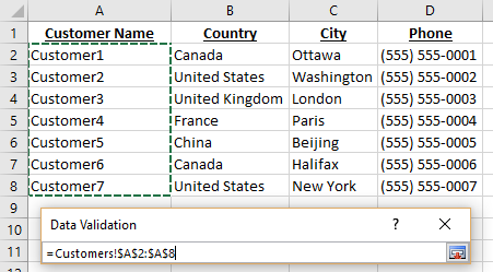
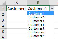
Adding an Excel Drop-down list is a great way to make data entry faster, more efficient, and also more accurate. There are a few ways they can be done, and in this article we show how to do them using the Data Validation lists.
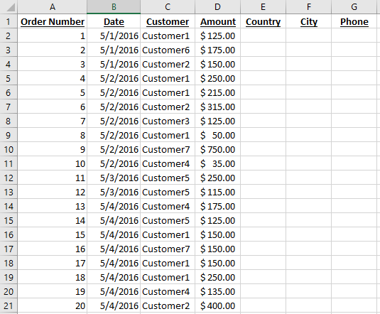
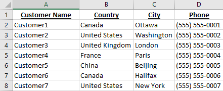
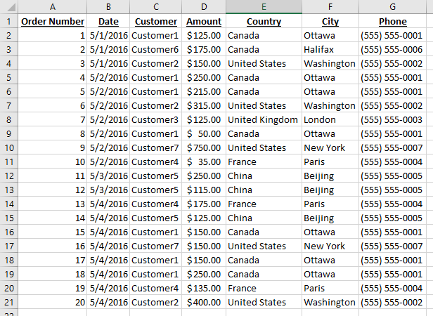
As an example of how the Excel Vlookup function works, let’s take a simple excel workbook with the following two tabs: Orders and Customers.
The Orders tab contains an order number, date, customer name, and amount.
We want to add the Country, City, and Phone number of each customer, which thankfully we have in the Customers tab.
By using the Excel VLOOKUP function, we can quickly and efficiently fill in the Country, City, and Phone in the Orders tab.
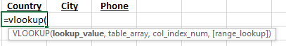
Let’s go back to the Orders tab, and start typing the =vlookup( formula to see the tooltip provided by Microsoft:
If you’ve never used the Excel vlookup function before, this provides absolutely no help. But lets break it down in an easier way:
Argument
Description
Example
Example Code
lookup_value
The value which is in common between both tables
In this case, Customer Name, more specifically, if we are trying to find the Country for the customer on line two (i.e. we are trying to fill cell E2), we would select cell C2 as the customer name.
C2
tabble_array
Where the information you are looking for is located. The first column should contain the common element, and the range should be large enough to include
In this case, it would be the Customers tab, columns A through D.
Customers!A:D
col_index_num
Based on the range you put in table_array, the col_index_num is the number of the column which contains the result you are looking for. For example, if you selected A:D as your range, and the common element is in column A, and the result is in column B, you would put 2 as your column number. Putting 3 would give you the result from column C, and putting 4 would give you the result from column D. However, if you select L:P as your range, then column 1 is L, column M is 2, column N is 3, etc.
Because the country code is located in column B of the Customers tab, we will select 2
2
[range_lookup]
Last and definitely not least, the range_lookup gives you a true or false option. False will only return an exact match, while True will try to look for a result which looks similar to what you are looking for. 99%+ of the time I find False to be the best option to use. For example, if you had an order for Customer8, because there is no Customer8 in the customers tab, using false would return #N/A meaning Excel could not find a match. This would let you know that you have to add Customer8 to the Customers tab. If you select true, that same Customer8 would return United States, because Customer8 looks similar to Customer7, which is in the US.
false
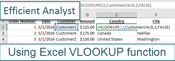
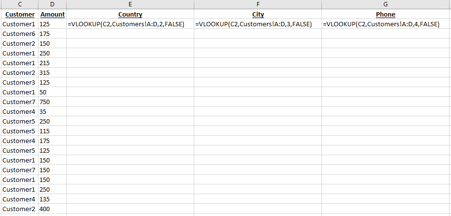
We end up with the following formula: =VLOOKUP(C2,Customers!A:D,2,FALSE), where C2 is the Customer we are trying to match up, Customers!A:D contains the customer information we want to look into, 2 is the 2nd column from that range, and False because we only want exact matches.
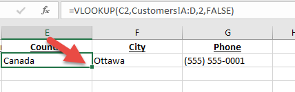
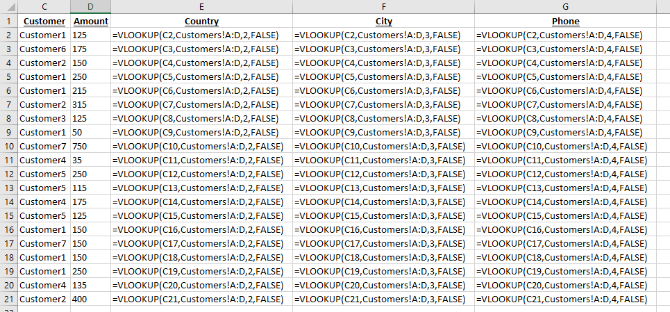
Using the same method, we can create the formulas for F2 and G2 by changing the 2 to a 3 or a 4. (I changed my view settings in Excel to show the formulas instead of the values, so you should see Canada, Ottawa, and (555) 555-0001 instead of the formulas)
You can then select a formula and drag the little dot in the corner to fill in the other formulas very quickly:
Which would give us the following formulas (again in formula view):
Here is what you should see on your screen at the end. By using the formula dragging feature, you can very quickly perform vlookups for thousands of records!
Additional Tips
Using full columns as your range, for example A:D instead of A2:D7, makes it easier to add/remove items from your table without having to change the 2 and 7 all the time.
If you do use a range such as A2:D7, remember that if you drag your formula down, you will get A3:D8, A4:D9, etc, and if you drag your formula right, you will get B2:E7, C2:F7, etc. The easiest way to prevent this is to use $ signs to make sure the range doesn’t change, such as $A$2:$D$7.
We use cookies to ensure that we give you the best experience on our website. If you continue to use this site we will assume that you are happy with it.


Recent Comments