Using a slicer, you can turn your dashboard into an interactive experience, enabling your users to quickly filter different values.
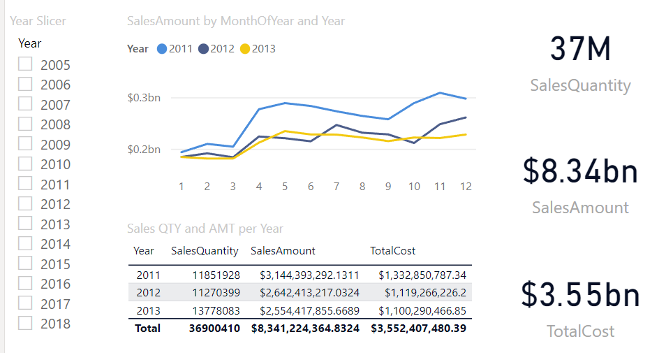
If you use a dimensional model as the source of your Power BI model, chances are at some point you will want to use a dimension such as your Calendar, Customer, or Production dimension to in a slicer to filter data on a page. For the most part, that will work well, but what if your Calendar dimension contains many more years of data than your Sales fact, such as in the example below?
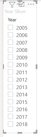
In this example, you will notice the Sales table only has sales for years 2011, 2012, and 2013, but the Year Slicer shows years from 2005 to 2018. While this can work, in this post we will show you how to clean this up to only show the years which have sales associate to them.
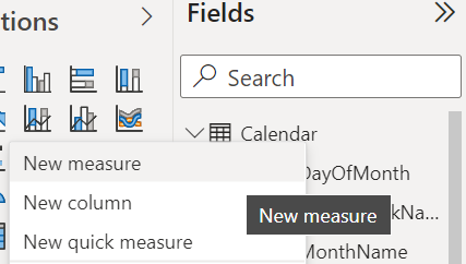
Create a New Measure in your Calendar Table
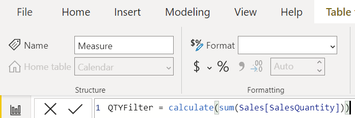
Using the Calculate() function, we will create a measure in the Calendar table that sums up the Sales Quantity per date. QTYFilter = calculate(sum(Sales[SalesQuantity]))
Right-click the Calendar table and select New Measure.
Type in the formula for the metric you want to filter by. In this case we will use the Sales Quantity: QTYFilter = calculate(sum(Sales[SalesQuantity])).
Use the QTYFilter Measure to Filter the Year Slicer
Select the Year slicer.
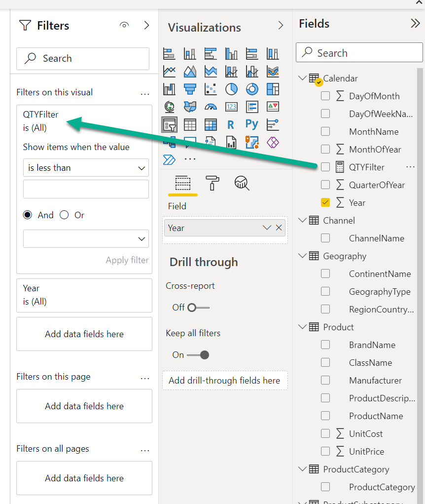
In the Filters pane, drag the QTYFilter measure to the Filters on this Visual section.
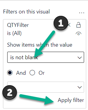
In the Drop Down box, select is not blank, and click Apply filter.
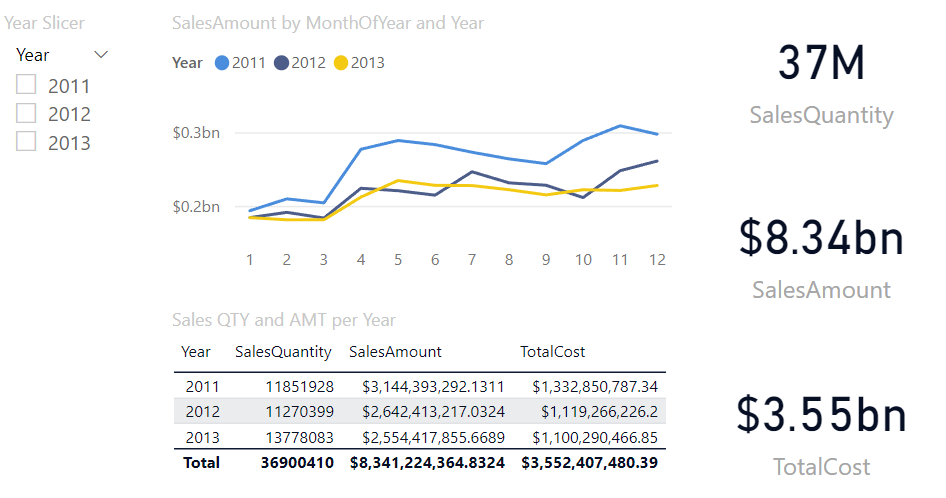
As you can see, the Year slicer now only contains years where there was a sales quantity, giving you a much cleaner slicer.
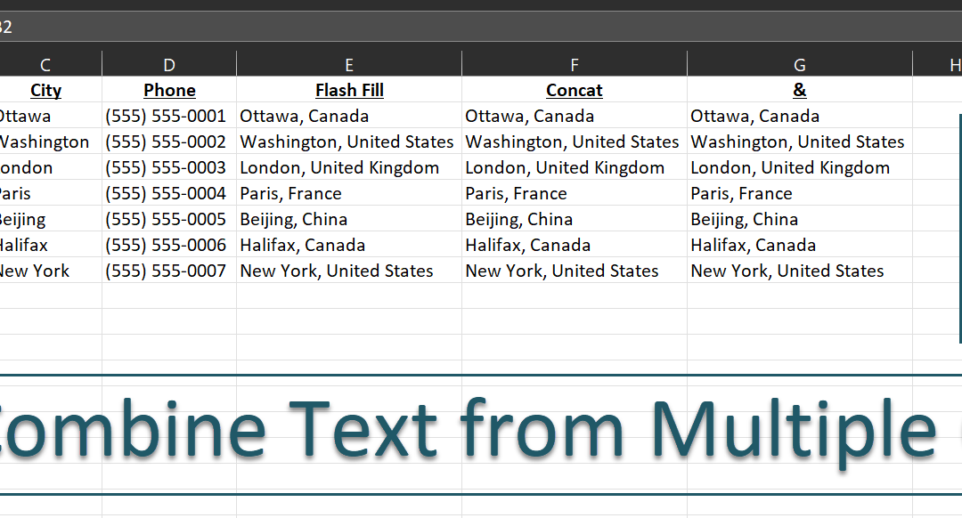
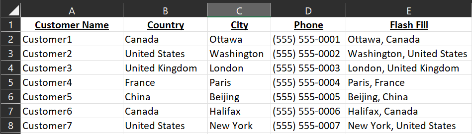
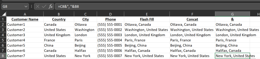
Today we will explore 3 ways of quickly combine text from multiple columns in Excel. In this example, we will combine the name of the City and the Country, while adding a comma in between. For example Ottawa, Canada.
Combine Text from Multiple Columns using Flash Fill
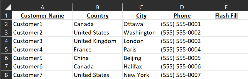
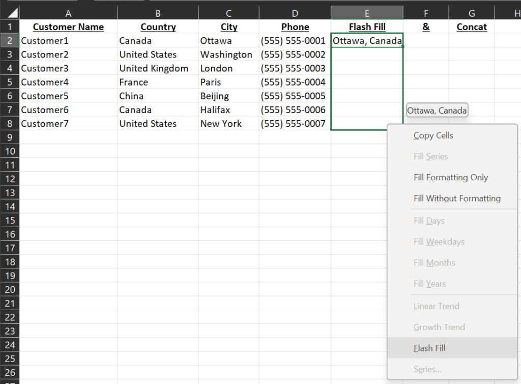
Excel 2013 introduced a new feature called flash fill, which seems to be getting better with every new release. Using the Customers – Exercise Book tab, we will be filling in column E, titled Flash Fill.
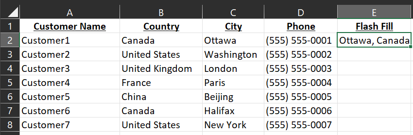
In cell E2, we will write the results how we would like to see them, in this case we will write Ottawa, Canada.
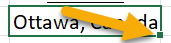
Next, we will select cell E2, and you can either press Control+E to fill in the rest of the column automatically, or you can right-click and hold the square in the bottom-right, and drag your mouse to the bottom of the table, as we can see here:
Select Flash Fill in the drop-down that appears. Excel’s AI will automatically fill in the rest.
Combine Text from Multiple Columns Using the Concat() function
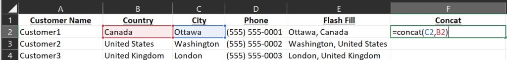
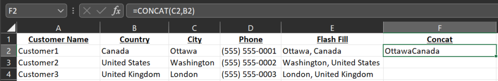
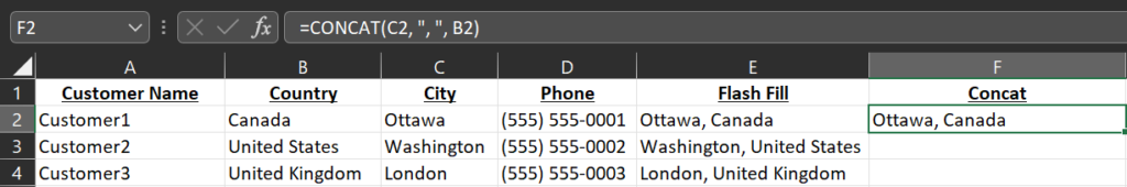
The Concat function can be used to combine data from multiple columns. In column F, we will do a quick formula to show how it works. We will start with concat(C2, B2), which will combine cells C2 and B2 together.
The end result is not quite what we want. As you can see, it squished both cells together, which we will fix next.
We will fix this by adding the text we want as a separator by using “, ” as follows: concat(C2, “, “, B2). As you can see, this formats the text as we expect it: Ottawa, Canada.
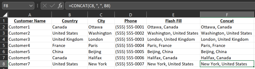
As always, you can drag the formula down by left-clicking the square in the bottom-right of cell F2 and dragging it to the bottom of the table to fill in the other cells automatically.
Combine Text from Multiple Columns Using &
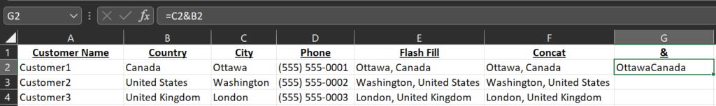
The last method we will see today is the one I actually use the most, which uses the & instead of the concat() function. To begin, in G2, we will write =C2&B2. Again you will notice that we get OttawaCanada all bunched up together. We will fix this in the next step.
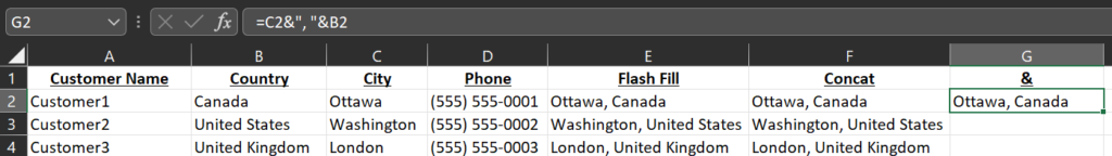
As we did with the concat() function, we will use “, ” to add a comma and a space between the City and Country, giving us the following formula: =C2&”, “&B2.
As always, you can left-click the square in the bottom right of the cell to drag down the formula to fill in the City, Country for the rest of the table.
We use cookies to ensure that we give you the best experience on our website. If you continue to use this site we will assume that you are happy with it.

Recent Comments