
Create Excel Pivot Table
When you know how to Create Excel Pivot Tables, you can quickly summarize data and gather additional insights.
To follow along, go to the following link to download the Efficient Analyst Pivot Table Exercise Book: https://efficientanalyst.com/wp-content/uploads/2022/01/Excel-Pivot-Table.xlsx
Procedure Steps
As an example of how the Excel Pivot Table feature works, let’s take a simple excel workbook with the following two tabs: Orders and Customers.

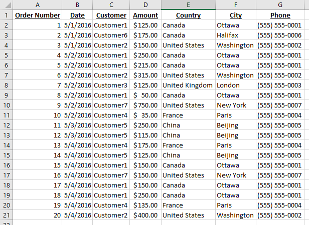
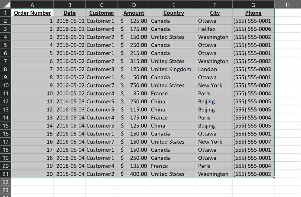
To begin, select the entire table, from cell A1 through to cell G21, or click on any cell within that range.
Or
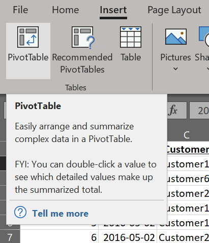
The Create PivotTable window will appear which shows the table/range that will be used as the input for the Pivot Table, and where you want the pivot table to be added.
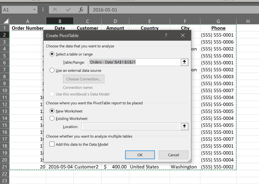
In this case, we will keep the default, and use New Worksheet. Press OK to continue.
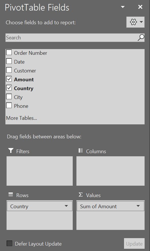
In the PivotTable Fields area, click and drag the Country field to the Rows section, and the Amount to the Values section. You will notice that Excel automatically notices the Amounts column contains numbers, so it will give you the sum.
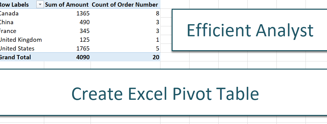
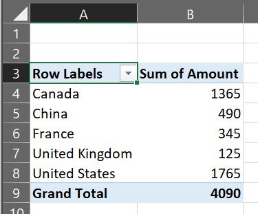
Notice the results are now displayed on the left.
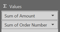
To add the count of orders, we will drag the Order Number field to the Values section also. Notice how Excel also detects the Order Number as a number, so chooses to aggregate with a sum. We will fix that shortly.
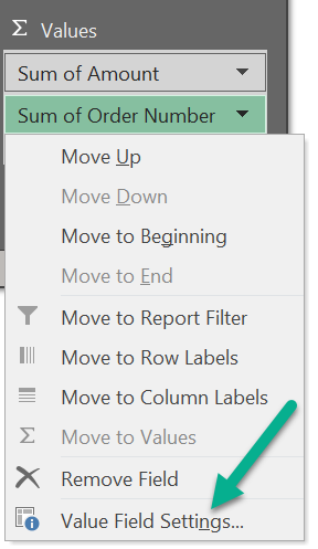
Click the triangle next to the Sum of Order Number, and select the Value Field Settings… menu option.
In the Value Field Settings window, select Count. This will rename the Custom Name as Count of Order Number.
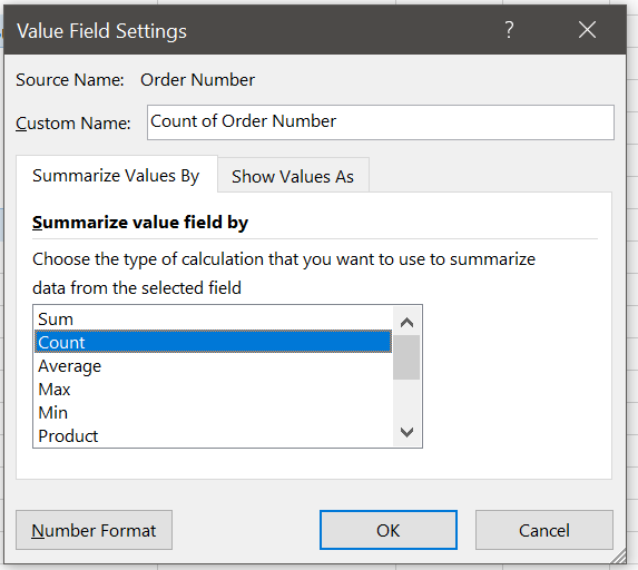
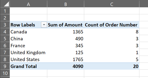
Click OK to apply the changes, and see the final results.
Recent Comments