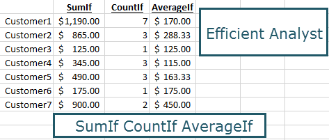
Excel SumIf CountIf and AverageIf formulas

by jplaforest | Mar 14, 2017 | Excel, Intermediate

Using Sum(), Count() and Average() formulas in Excel might be enough for many situations, but sometimes you might have a more complex question you’re trying to answer.  For example, if you had the following data, and you wanted to know how much each customer bought, how many times they bought, and what was their average purchase, you will need a new set of formulas.  Don’t worry, though, you’ll see they are just as easy to use. The Excel SumIf(), CountIf() and AverageIf() formulas will give you the sum, count, and average of a value where a certain condition is matched.

To follow along, go to the following link to download the Efficient Analyst SumIf CountIf AverageIf Exercise Workbook:

Efficient Analyst Excel SumIf CountIf AverageIf

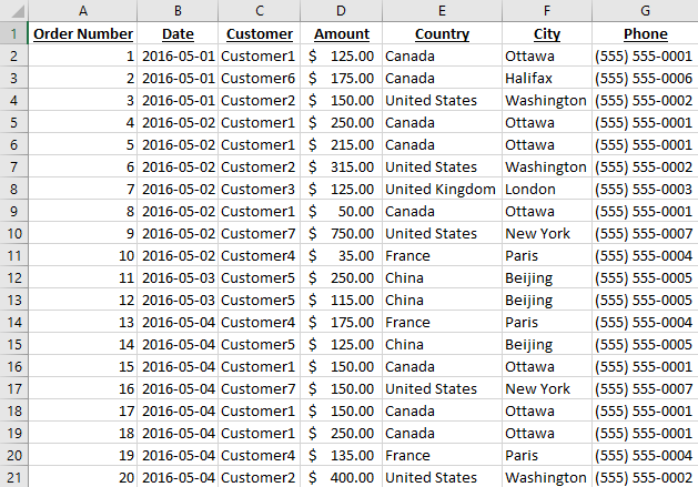
First, lets look at our sales data.  You might recognize this from a previous exercise.

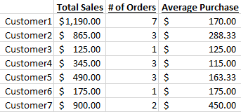
What you are looking for is a simple table as follows, so you can start learning more who your best customers are, and some of their buying habits.

Let’s see which functions will give us the right information for each column:

Using the Excel SumIf Formula

If you start writing =SumIf( in Excel, a tooltip will appear which gives you a reminder of how to use this formula.

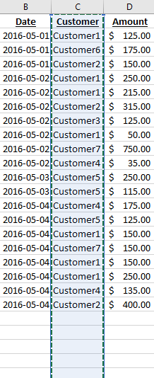
The first part you will need to fill out is the range.  In this case, the range will can be thought of as “Where do you want to look for this customer name?”, the answer being column C, which in Excel you can either click the column C header to select it, or write C:C. Let’s click the column header to select it:

Also notice how the formula updated.

The second section we have to fill is the criteria. The criteria is what you are trying to match, which in this case is Customer 1, which is found in cell I2, so we will select I2.

Last but not least, we need to tell Excel what we need to sum, the sum range, which in this case would be the amounts found in column D.

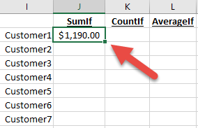
Congratulations, you know know how to use SumIf!. If you close the parenthesis ) of the formula and press enter, you will see how much Customer1 has purchased:

Dragging Down a Formula to Copy it Over a Range

One of my favourite features of Excel is the ability to drag a formula down to copy it quickly over a range. Select the cell containing your SumIf formula, and then click and hold your left mouse button on the the little dot in the bottom right of that cell.

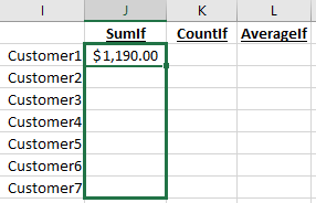
While keeping your left mouse button pressed down, move your mouse cursor down over the area you would like to copy this formula to.

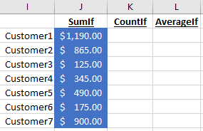
Release the left mouse button, and you will see the formula copied itself over making adjustments as needed so the formula in cell J3 is matching the content in cell I3, etc.

Using the Excel CountIf Formula

To find out how many times each customer placed an order, we will use the CountIf formula, which counts how many times some text appears in your selection. This formula is a little simpler than the other two, having only two sections: a range, and a criteria.

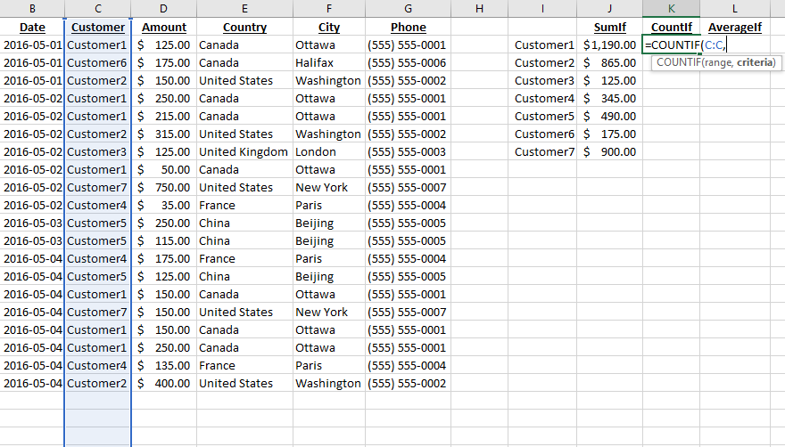
The first step consists in writing =countif( to see the Excel tooltip.

The range comes first, which is where you want to look for a match, which in this case would be column C. You can either select column C, or write C:C in the formula bar.

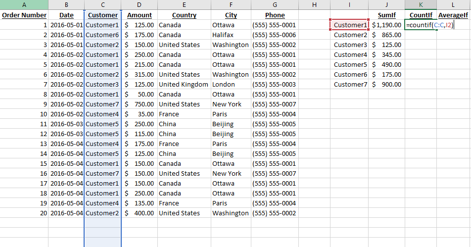
Next up is the criteria which is what we are trying to match, which in this case would be the content of cell I2.

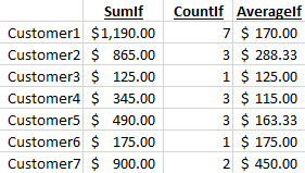
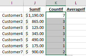
Closing the parenthesis ), pressing enter, and then using the dragging technique from before, we get the number of purchases per customer.

Using the AverageIf Excel Formula

To obtain the average sales amount per order, we have two options. Since we already calculated the sum of the amounts and the count of orders, we could simply go in cell L2 and type =J2/K2. But since this is a tutorial, let’s use this exercise as an excuse to learn AverageIf, that way you don’t have to use SumIf and CountIf if all you’re looking for is the average.

As usual, type =averageif( in a cell will give you the tooltip on how to use this tool. If you look at the 3 arguments of this formula: range, criteria, and average range, you’ll notice this follows the same structure as the SumIf() formula we have just seen.

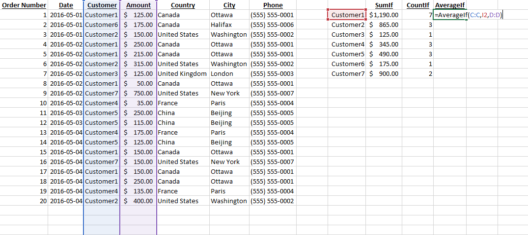
Using a range of column C, a criteria of cell I2, and an average range of column D, we get the following formula:

Using the same drag-down technique as before, we get the average sales per customer.